Hypothesis test

Hypothesis test about fine amount

Anova between fine amount and different boros

From data exploration, we have notice that the violation code varies among boroughs as well as the fine amount. We see from the table that the mean of fine amount in Queen is different from the Manhattan by 10$, and thus, we propose hypothesis that there’s at least 1 pairs of boroughs’ fine amount is different from others.

Fine Amount in borough
borough	mean	standard_error
Bronx	75.8	35.3
Brooklyn	70.5	33.2
Manhattan	82.0	34.3
Queens	66.2	33.7
Staten Island	77.8	31.2

To do that, we perform ANOVA test for multiple groups comparison. With:

$H_0$ : there’s no difference of fine amount means between boroughs

$H_1$ : at least two fine amount means of boroughs are not equal

##                      Df   Sum Sq  Mean Sq F value Pr(>F)    
## factor(borough)       4 9.24e+07 23099132   19954 <2e-16 ***
## Residuals       2235719 2.59e+09     1158                   
## ---
## Signif. codes:  0 '***' 0.001 '**' 0.01 '*' 0.05 '.' 0.1 ' ' 1

Turkey Test at 99% confidence Level
	diff	lwr	upr
Brooklyn-Bronx	-5.24	-5.50	-4.99
Manhattan-Bronx	6.18	5.95	6.42
Queens-Bronx	-9.61	-9.87	-9.36
Staten Island-Bronx	2.05	1.36	2.75
Manhattan-Brooklyn	11.43	11.23	11.62
Queens-Brooklyn	-4.37	-4.59	-4.15
Staten Island-Brooklyn	7.29	6.61	7.97
Queens-Manhattan	-15.80	-16.00	-15.60
Staten Island-Manhattan	-4.13	-4.81	-3.46
Staten Island-Queens	11.67	10.98	12.35

As the ANOVA test result from above, we reject the Null at 99% confidence level and conclude that there’s at least one borough’s mean of fine amount is different from others.

To further investigate the difference between boroughs, we perform Tukey test for pairwise comparison. Notice that all paris are different from each other in the setting of our data. Given the large amount of data, according to the law of large number, the estimate of mean fine amount close to the true mean of the fine amount in different borough. Under this setting, we have 99% confidence that Manhattan have different mean of fine amount than other borough. So if you unfortunately get a RISKY coffee, it is much burning than in other boroughs.

Hypothesis test about violation counts

Chi-Squared test between violation counts generated in each weekdays and different boroughs

From data exploration, we have noticed that the violation counts proportions in different weekdays among each boroughs are different.Thus, we assume there is no homogeneity in tickets counts proportions in each weekdays among boroughs.

To verify that, we performed Chi-squared test for multiple groups comparison. With:

$H_0$ : the tickets proportion in weekdays among boroughs are equal.

$H_1$ : not all proportions are equal

Test Result
	Monday	Tuesday	Wednesday	Thursday	Friday	Saturday	Sunday
Bronx	40042	48014	52401	63138	58693	26226	11314
Brooklyn	70543	89805	91964	113167	101244	38505	17231
Manhattan	129973	155645	164414	180871	163717	71638	32421
Queens	71468	81945	87930	97113	88915	46276	13338
Staten Island	4768	4940	5094	5568	5005	1920	597

## 
##  Pearson's Chi-squared test
## 
## data:  chisq_boro_day
## X-squared = 4609, df = 24, p-value <2e-16

According to above chi-square test result and the x critical value ( = 36.415) We reject the null hypothesis and conclude that there’s at least one borough’s proportions of violation counts for week days is different from others at 0.05 significant level.

Chi-Squared test between violation counts generated in each hour and different boroughs:

	0	1	2	3	4	5	6	7	8	9	10	11	12	13	14	15	16	17	18	19	20	21	22	23
Bronx	2480	2424	1658	1100	155	4091	21193	24695	42396	31769	25924	31483	31354	21105	17330	10662	9886	4356	1449	630	3697	4472	3256	2263
Brooklyn	5036	6226	4399	2635	2466	8856	13948	33412	59796	62194	37938	67174	56173	46268	35120	27595	17509	11708	6128	1276	4278	5318	4233	2773
Manhattan	1879	1753	1767	1088	318	2918	19570	67369	107663	97228	83393	81212	74025	124636	87194	53599	36714	32399	9463	1689	4145	3539	2697	2421
Queens	1588	2358	1932	1191	661	4464	21283	27877	62299	58735	41416	49727	41718	45968	42111	21688	26317	18371	5915	355	1830	3696	3436	2049
Staten Island	63	213	167	116	59	73	758	3531	3275	2802	2057	1373	497	2482	3125	2548	2025	1332	611	118	147	208	186	126

statistic	p.value	parameter	method
110937	0	92	Pearson’s Chi-squared test

According to above chi-square test result and the x critical value ( = 115.39), We reject the null hypothesis and conclude that there’s at least one borough’s proportions of violation counts for 24 hours is different from others at 0.05 significant level.

Sine 526.14 million square feet of office space existed in Manhattan in 2020. Manhattan’s office space is located in 3,830 commercial buildings in the major markets of Midtown, Midtown South, Lower Manhattan and Uptown [Statistics]. At any given time most of this office space is rented. Manhattan becomes the well deserved business center in NYC. Due to the unequal active status of commerce among boroughs and expensive costs of keeping a car in NYC, the active area of life and work for people who own a car concentrates upon Manhattan. This is one of reasonable explanations of chi-square test result. But this situation might be changed since the commercial areas tend to extend to other boroughs. Some data in the report shows that the Bronx office market and the Staten Island office market have seen increased investor interest over the past 10 years [click here to get more detailed information].

Regression Exploration

The resulting data frame of boro_daytime_violation contains a single dataframe df with 2,231,935rows of data on 8 variables, the list below is our variables of interest:

violation_number. mean of violation
month. Issue month
workday_weekend. a factor variable: 1 represent workday(Monday to Friday), 0 represent weekend
hour. Time(hour) violation occurred.
daytime. a factor variable: 1 represent daytime(8am to 8pm), 0 represent night(8pm to 8am)
street_name. Street name of summons issued.
vehicle_color. Color of car written on summons.
borough. Borough of violation.

The data frame of boro_daytime_violationln contains an addtional variable:

ln_violation. logarithm transformation of mean of violation

boro_daytime_violation = 
  parking %>%  
  mutate(
    daytime = if_else(hour %in% 8:20,"1","0"),
    day_week = weekdays(issue_date),
    workday_weekend = if_else(day_week %in% c("Monday", "Tuesday", "Wednesday","Thursday", "Friday"),"1","0"),
    month = lubridate::month(issue_date),
    month = forcats::fct_reorder(as.factor(month),month)
  ) %>% 
  drop_na(vehicle_color, street_name) %>% 
  group_by(borough,month,workday_weekend,daytime) %>%
  summarise(
    violation_number = mean(n()),
    street_name = street_name,
    vehicle_color = vehicle_color,
    street_name = street_name,
    month = month,
    hour = hour
  )

Box-Cox Transformation

fit1 = 
  lm(violation_number ~ borough + factor(workday_weekend) + factor(daytime) + month, data = boro_daytime_violation)
MASS::boxcox(fit1)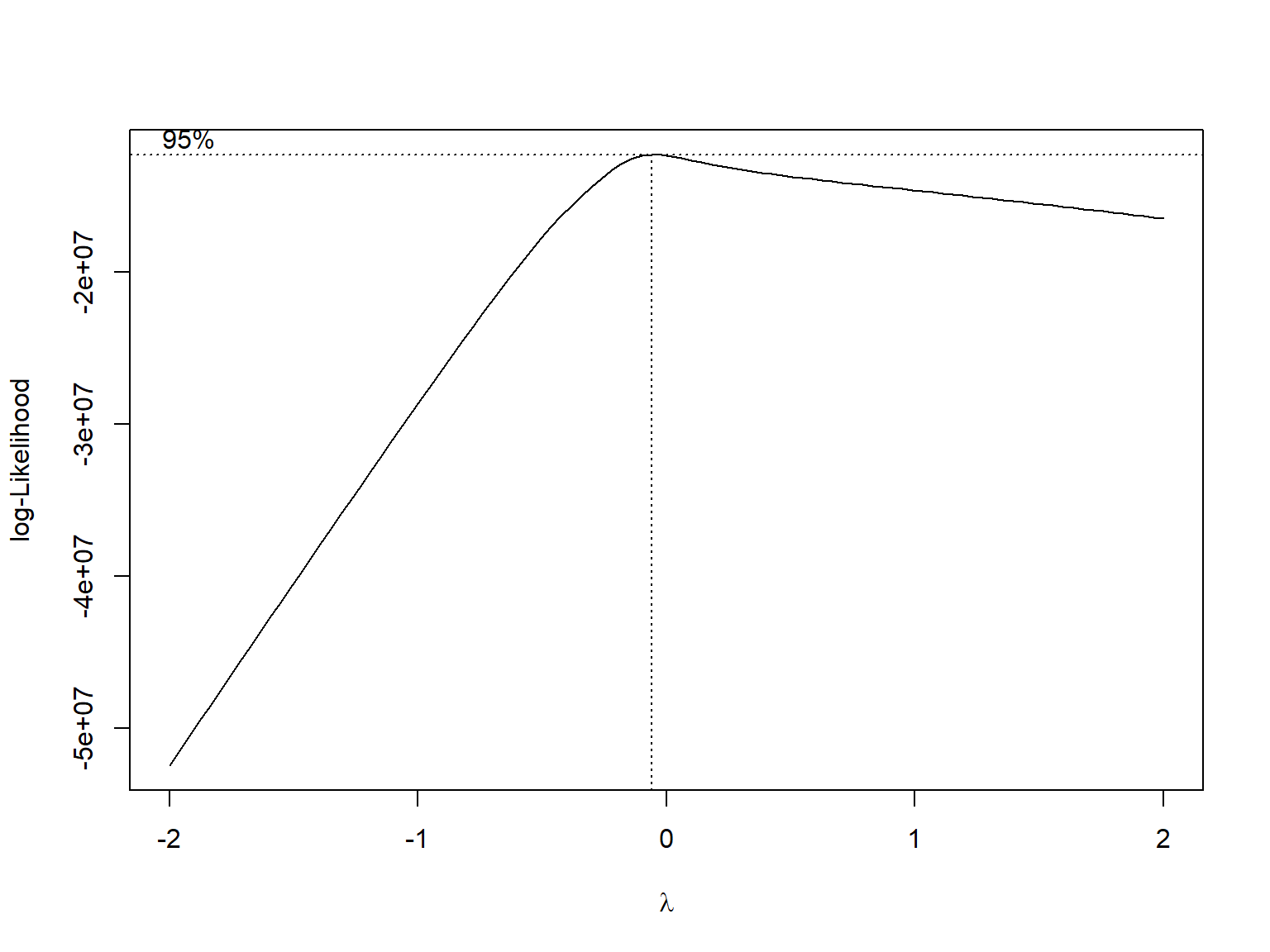

we use box-cox method to determine transformation of y. Since λ is close to 0, logarithm transformation should apply to violation counts.

MLR

boro_daytime_violationln = boro_daytime_violation %>%
  mutate(ln_violation = log(violation_number, base = exp(1)))
fit1 = 
  lm(ln_violation ~ borough + factor(workday_weekend) + factor(daytime) + month, data = boro_daytime_violationln)
fit1 %>% 
  broom::tidy() %>% 
  mutate(
    term = str_replace(term, "borough", "Borough: "),
    term = str_replace(term, "month", "Month: "),
    term = str_replace(term, "factor(workday_weekend)1", "workday "),
    term = str_replace(term, "factor(daytime)1", "daytime(8am to 8pm) ")
  ) %>% 
  knitr::kable(caption = "Linar Regression Result")

Linar Regression Result
term	estimate	std.error	statistic
(Intercept)	-2.355	0.041	-57.02
Borough: Brooklyn	0.535	0.000	1367.79
Borough: Manhattan	1.080	0.000	2989.61
Borough: Queens	0.459	0.000	1158.42
Borough: Staten Island	-2.381	0.001	-2204.74
factor(workday_weekend)1	1.987	0.000	5549.69
factor(daytime)1	1.681	0.000	5233.50
Month: 2	0.769	0.048	15.87
Month: 3	1.378	0.045	30.66
Month: 4	0.657	0.049	13.34
Month: 5	2.633	0.042	62.36
Month: 6	7.457	0.041	180.54
Month: 7	9.507	0.041	230.21
Month: 8	10.091	0.041	244.33
Month: 9	10.011	0.041	242.39
Month: 10	0.289	0.057	5.08
Month: 11	0.641	0.127	5.04

From above linear regression model, we could see that boroughs, month, workday/weekend, daytime/night are significant variables for violation counts prediction in comparison to the reference group.

$~$ When Bronx works as reference, the p values for “Brooklyn”, “Manhattan”, “Queens” are far away smaller than 0.05. This means boroughs has significant effect on violation counts prediction. Staten Island has negative estimate and very small p value because its very small violation counts by comparing to other boroughs.

$~$

The NYC parking regulation:free parking on major Legal Holidays and Sundays:. This explain why p-value of workday is below 0.05 when weekend as reference. That means workday factor is significant. Comparing with weekend, there are more parking violation on workdays than weekend due to NYC free parking rules on Sunday.This result is corresponding with the Violation per Hour plot we made in data exploration

$~$

The p vale of daytime is less than 0.05. It makes sense, since people more likely to go out and parking on the street on daytime than night. And parking seems to become a routine issue for commuters.

$~$

The P value for each month is smaller than e^6. No matter which month to go out, there will be a significant risk of receiving a parking tickets. The police goes to work on the whole of the year. There might have another explanation for the significance of month. There might some months need to be pay more attention to. May, June, Junly and August are usually summer holiday for students all over the world. Due to that NYC is a tourist attraction, the number of tourists should be increased from May to August. Tourists who aren’t familiar with the NYC parking rules may easily receive parking tickets.

Model diagnosis

summary(fit1)

## 
## Call:
## lm(formula = ln_violation ~ borough + factor(workday_weekend) + 
##     factor(daytime) + month, data = boro_daytime_violationln)
## 
## Residuals:
##    Min     1Q Median     3Q    Max 
## -2.725 -0.056  0.026  0.048  3.967 
## 
## Coefficients:
##                           Estimate Std. Error  t value Pr(>|t|)    
## (Intercept)              -2.354896   0.041300   -57.02  < 2e-16 ***
## boroughBrooklyn           0.534709   0.000391  1367.79  < 2e-16 ***
## boroughManhattan          1.080457   0.000361  2989.60  < 2e-16 ***
## boroughQueens             0.459405   0.000397  1158.42  < 2e-16 ***
## boroughStaten Island     -2.381006   0.001080 -2204.74  < 2e-16 ***
## factor(workday_weekend)1  1.987414   0.000358  5549.69  < 2e-16 ***
## factor(daytime)1          1.680710   0.000321  5233.50  < 2e-16 ***
## month2                    0.769229   0.048476    15.87  < 2e-16 ***
## month3                    1.378417   0.044952    30.66  < 2e-16 ***
## month4                    0.657425   0.049299    13.34  < 2e-16 ***
## month5                    2.632771   0.042217    62.36  < 2e-16 ***
## month6                    7.457171   0.041304   180.54  < 2e-16 ***
## month7                    9.507427   0.041299   230.21  < 2e-16 ***
## month8                   10.090537   0.041299   244.33  < 2e-16 ***
## month9                   10.010605   0.041299   242.39  < 2e-16 ***
## month10                   0.288700   0.056847     5.08  3.8e-07 ***
## month11                   0.641279   0.127291     5.04  4.7e-07 ***
## ---
## Signif. codes:  0 '***' 0.001 '**' 0.01 '*' 0.05 '.' 0.1 ' ' 1
## 
## Residual standard error: 0.17 on 2231825 degrees of freedom
## Multiple R-squared:  0.98,   Adjusted R-squared:  0.98 
## F-statistic: 6.72e+06 on 16 and 2231825 DF,  p-value: <2e-16

set.seed(500)
sample_fit1 = 
  boro_daytime_violationln %>% 
  sample_n(5e+3, replace = TRUE)

sample_lm = lm(ln_violation ~ borough + factor(workday_weekend) + factor(daytime) + month, sample_fit1)
par(mfrow = c(2,2))
plot(sample_lm)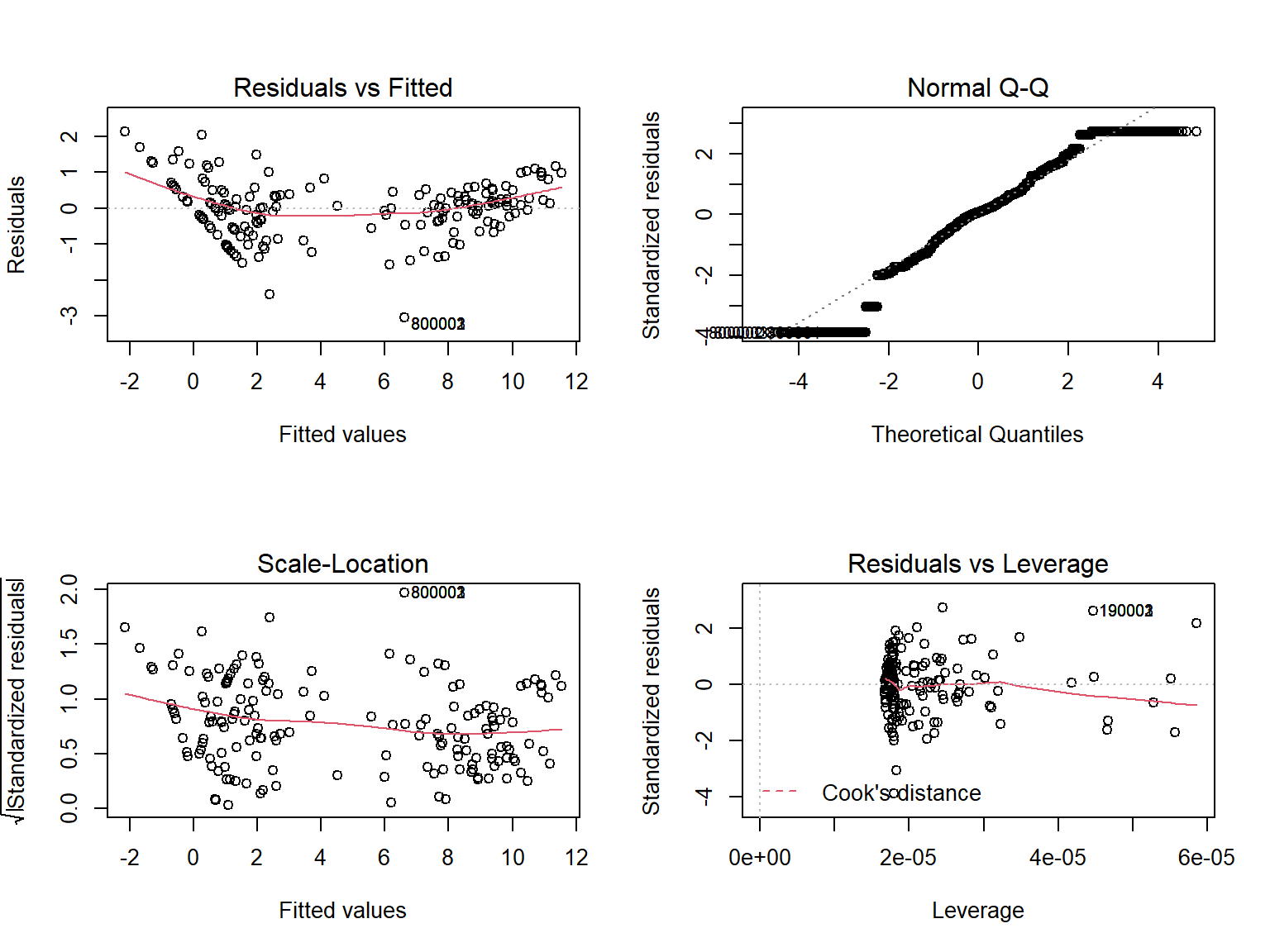

We can see that the residual vs fitted is not equally distributed around 0 horizontal line. In fact, there’s a pattern in the residual, indicating that the model although have high goodness of fit, but violating normal assumption on the residual. As a matter of fact, our data follows poison distribution, and thus linear model wouldn’t be appropriated for our model. When we doing regression, linear model will not be consider.